
Goal: In this lesson, we’ll learn every stage of the Machine Learning lifecycle, understand what happens at each step, and see how MLOps automates and manages the entire process.
Difficulty: Beginner → Early Intermediate
Estimated Time: 90–120 minutes
By the end of this lesson, you should be able to:
             Business Problem
                    │
                    ▼
             Data Collection
                    │
                    ▼
             Data Validation
                    │
                    ▼
           Data Preparation
                    │
                    ▼
          Feature Engineering
                    │
                    ▼
            Model Training
                    │
                    ▼
            Model Evaluation
                    │
           ┌────────┴────────┐
           │                 │
       Reject           Register Model
                             │
                             ▼
                     Model Deployment
                             │
                             ▼
                     Production Serving
                             │
                             ▼
                     Model Monitoring
                             │
                             ▼
                    Continuous Retraining
                             │
                             └──────────────► Back to Training
Unlike traditional software, this is a continuous feedback loop, not a one-time process.
Every ML project starts with a business objective, not a model.
Poor Objective
Build an AI model.
Better Objective
Reduce customer churn by 10%.
Best Objective
Predict customers likely to cancel their subscription within the next 30 days with at least 90% precision.
Notice that the last objective is measurable.
Suppose you’re building a fraud detection system.
Business question:
Can we identify fraudulent transactions
before payment completes?
Possible ML task:
Binary Classification
Fraud OR Not Fraud
Machine learning systems are only as good as the data they learn from.
Data may come from:
Example:
Customer Purchase Table

Customer_ID
Age
Location
Orders
Items
Total
Payment_Type
Fraud_Label
Real Production Challenge
Data often contains:
MLOps pipelines automate data quality checks before training begins.
Before training, validate that the data meets expectations.
Examples:
Example Check
Expected:
Age
Integer
0–120Received:
Age
Twenty Five
Training should fail because the schema is invalid.
Raw data collected from databases, APIs, application logs, sensors, or other sources is rarely suitable for direct use in model training. Real-world datasets often contain missing values, duplicate records, inconsistent formats, incorrect data types, and features that machine learning algorithms cannot process directly.
Data preparation transforms this raw data into a clean, consistent, and model-ready dataset.
Common Data Preparation Steps
| Step | Purpose | Example |
|---|---|---|
| Remove duplicates | Prevent repeated records from unnecessarily influencing the model | Remove duplicate customer transactions |
| Handle missing values | Deal with incomplete records | Replace a missing age with the median age |
| Normalize numerical features | Bring numerical values to a comparable scale | Convert income values to a standardized range |
| Encode categorical variables | Convert non-numerical categories into a machine-readable representation | Convert Male/Female into numerical values |
| Split the dataset | Create separate datasets for training and unbiased evaluation | ~70% training, ~15% validation, ~15% testing |
Example: Encoding Categorical Data
Many machine learning algorithms require numerical inputs. Therefore, categorical values may need to be converted into an appropriate numerical representation.
After encoding, the model receives numerical values instead of text:
Before Encoding             After Encoding

Gender                         Gender
──────                         ──────
Male                              0
Female                            1
Female                            1
Male                              0
However, Male → 0 and Female → 1 does not mean that one category is mathematically greater than the other. The numbers are simply representations of categories.
A feature is an input variable that a machine learning model uses to identify patterns and make predictions.
The data available in its original form is not always the most useful representation for a model. Feature engineering is the process of transforming existing raw data into more meaningful variables that better represent the underlying business problem.
In simple terms:
Raw data tells us what happened. Well-designed features help the model understand what that data means.
Suppose a customer dataset contains:
| Customer | Date of Birth |
|---|---|
| Customer A | 15 March 1990 |
| Customer B | 8 August 1985 |
The raw Date of Birth may not be directly useful to many machine learning algorithms. Instead, we can derive a more meaningful feature:
Date of Birth
      ↓
Feature Engineering
      ↓
     Age
The resulting dataset might look like:
| Customer | Date of Birth | Age |
|---|---|---|
| Customer A | 15 March 1990 | 36 |
| Customer B | 8 August 1985 | 40 |
If we are building a model to predict customer purchasing behavior, Age may provide a more directly useful signal than the original date of birth.
Consider raw transaction data:
| Customer | Month | Purchase Amount |
|---|---|---|
| Customer A | January | ₹10,000 |
| Customer A | February | ₹15,000 |
| Customer A | March | ₹20,000 |
nstead of passing every individual transaction directly to the model, we can derive behavioral features such as:
Average Monthly Spend = ₹15,000
From the same purchase history, we could potentially create several features:
These derived features summarize customer behavior in a form that the model can learn from more effectively.
Suppose you are building a model to predict whether a customer will stop using a service.
The raw dataset may contain thousands of individual login records. Rather than giving the model only those raw records, you could derive:
| Raw Data | Engineered Feature | Potential Signal |
|---|---|---|
| Login timestamps | Logins in the last 30 days | Recent engagement |
| Transaction history | Average monthly spend | Customer value |
| Account creation date | Account age | Customer maturity |
| Support tickets | Tickets in the last 90 days | Customer dissatisfaction |
| Subscription history | Number of plan changes | Behavioral instability |
A feature such as “days since last login” may provide a much stronger predictive signal for customer churn than the original login timestamps.
This is why feature engineering can sometimes improve model performance more than simply replacing one algorithm with another. A sophisticated algorithm trained on poorly represented data may perform worse than a simpler algorithm trained on highly informative features.
However, feature engineering must be performed carefully. Features should be available at prediction time and must not contain information from the future; otherwise, data leakage can occur and produce unrealistically high evaluation results.
The algorithm determines how the model learns. Feature engineering determines what useful information the model has available to learn from.
Once the data has been cleaned, transformed, and divided into training and evaluation datasets, the next stage is model training.
Model training is the process in which a machine learning algorithm analyzes the training data and learns the statistical relationships between input features (X) and the corresponding target variable (y).
For example, consider an email spam classification problem.
| Email Features (X) | Target (y) |
|---|---|
| Number of suspicious links, sender reputation, keyword frequency | Spam |
| Number of suspicious links, sender reputation, keyword frequency | Not Spam |
During training, the algorithm attempts to learn patterns that distinguish spam emails from legitimate emails.
A simple example using a Random Forest classifier:
from sklearn.ensemble import RandomForestClassifier

# Initialize the model
model = RandomForestClassifier(
    n_estimators=100,
    random_state=42
)

# Train the model
model.fit(X_train, y_train)
Here, X_train contains the input features used for learning, while y_train contains the correct target values or labels associated with those observations to the selected learning algorithm.
Conceptually, the training process/program looks like this:
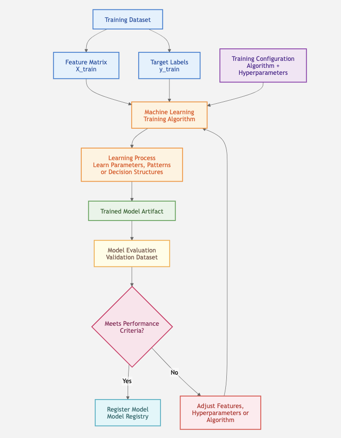
The exact training process depends on the type of algorithm being used. For a Random Forest, the algorithm:
The result is a trained model that has learned decision patterns from historical data.
For example, the model might learn relationships such as:
Many suspicious links
        +
Poor sender reputation
        +
High frequency of spam-related terms
        ↓
Higher probability of SPAM
These rules are learned from the data rather than manually programmed by a developer.
Parameters vs. Hyperparameters
An important distinction in model training is between model parameters and hyperparameters.
| Type | Meaning | Random Forest Example |
|---|---|---|
| Parameters | Values learned automatically during training | Decision rules and split thresholds inside trees |
| Hyperparameters | Configuration values specified before training | Number of trees, maximum tree depth, minimum samples per split |
For example:
model = RandomForestClassifier(
    n_estimators=200,
    max_depth=10,
    min_samples_split=5
)
These values control how the model is trained, but they are not directly learned from the training data.
After training is complete, the model can receive previously unseen feature values and generate predictions. However, successful training alone does not mean the model is production-ready. The next stage is model evaluation, where its ability to generalize to unseen data is measured.
Training Is Often an Experimental Process
A single training run does not necessarily produce the best model. Data scientists commonly train multiple model candidates using different algorithms, feature combinations, and hyperparameter configurations.
For example:
Experiment 1 → Random Forest → Accuracy: 91%
Experiment 2 → XGBoost → Accuracy: 94%
Experiment 3 → Neural Network → Accuracy: 92%
Each training run should be recorded using an experiment tracking system so that results can be compared and reproduced.
The best-performing model is not automatically deployed to production. It must first pass the required evaluation and validation criteria defined by the organization.
Model training should be treated as a reproducible and traceable pipeline rather than a one-time execution of a machine learning algorithm.
A model that trains successfully is not automatically ready for production. Before deployment, it must be evaluated on unseen data to determine whether it can generalize beyond the examples used during training.
In an MLOps workflow, model evaluation acts as a quality gate:
Trained Model → Evaluate on Unseen Data → Check Metrics → Approve or RejectTraining vs. Validation Performance
Consider the following results:
| Dataset | Accuracy |
| Training Data | 99% |
| Validation Data | 81% |
The significant difference between training and validation performance is known as a generalization gap and may indicate overfitting.
The model has learned the training data extremely well but does not perform equally well on new data.
However, a large performance gap should be investigated rather than automatically classified as overfitting. Dataset shift, data leakage, inconsistent preprocessing, or an unrepresentative validation dataset can produce similar behavior.
Choosing the Right Evaluation Metric
The appropriate metric depends on the type of machine learning problem and its business requirements.
| Problem Type | Common Metrics |
| Classification | Accuracy, Precision, Recall, F1-score, ROC-AUC |
| Regression | MAE, MSE, RMSE, R² |
For classification problems, accuracy alone is often insufficient, particularly when the dataset is imbalanced.
For example, in fraud detection, missing an actual fraudulent transaction may be significantly more costly than incorrectly flagging a legitimate transaction. In such cases, recall may be more important than overall accuracy.
The evaluation metric should therefore reflect the actual business objective and the cost of prediction errors.
Model Evaluation as an MLOps Quality Gate
Production MLOps pipelines should define measurable acceptance criteria for model promotion.
For example:
F1-score ≥ 0.90
Recall ≥ 0.95
ROC-AUC ≥ 0.92
The pipeline can then automatically determine whether a model is eligible to move forward:
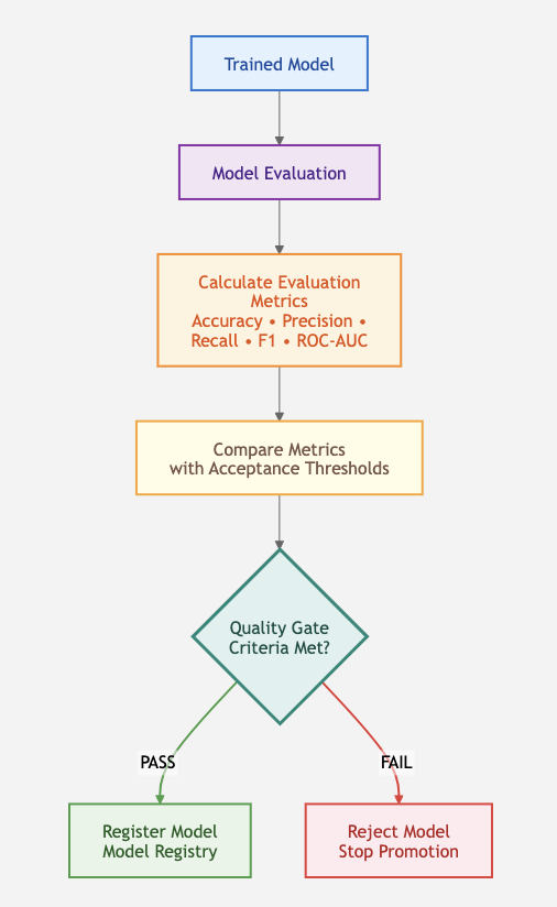
This transforms model evaluation from a manual activity into a repeatable and automated MLOps process.
Python Example: Evaluating a Classification Model
Sample Project Structure:
mlops-project/
│
├── data/
│   ├── train.csv
│   └── validation.csv
│
├── artifacts/
│   ├── model.joblib
│   └── evaluation_metrics.json
│
├── src/
│   ├── train.py
│   └── evaluate.py
│
└── requirements.txt
Model Training: The training component trains the model and persists it to an artifact store or shared pipeline location.
from pathlib import Path

import joblib
import pandas as pd
from sklearn.ensemble import RandomForestClassifier


# ---------------------------------------------------------
# Configuration
# ---------------------------------------------------------

TRAIN_DATA_PATH = Path("data/train.csv")
MODEL_OUTPUT_PATH = Path("artifacts/model.joblib")

TARGET_COLUMN = "target"


# ---------------------------------------------------------
# Load training data
# ---------------------------------------------------------

print("Loading training data...")

train_data = pd.read_csv(TRAIN_DATA_PATH)

X_train = train_data.drop(columns=[TARGET_COLUMN])
y_train = train_data[TARGET_COLUMN]

print(f"Training samples: {len(X_train)}")
print(f"Number of features: {X_train.shape[1]}")


# ---------------------------------------------------------
# Initialize the model
# ---------------------------------------------------------

model = RandomForestClassifier(
    n_estimators=100,
    max_depth=10,
    random_state=42
)


# ---------------------------------------------------------
# Train the model
# ---------------------------------------------------------

print("Starting model training...")

model.fit(X_train, y_train)

print("Model training completed.")


# ---------------------------------------------------------
# Save the trained model artifact
# ---------------------------------------------------------

MODEL_OUTPUT_PATH.parent.mkdir(
    parents=True,
    exist_ok=True
)

joblib.dump(
    model,
    MODEL_OUTPUT_PATH
)

print(f"Model artifact saved: {MODEL_OUTPUT_PATH}")
The output of this stage is: artifacts/model.joblib . This file represents the trained model artifact and becomes the input to the evaluation stage.
Model Evaluation: The evaluation process runs independently and loads the model artifact produced by the training stage.
from pathlib import Path
import json

import joblib
import pandas as pd

from sklearn.metrics import (
    accuracy_score,
    precision_score,
    recall_score,
    f1_score,
    roc_auc_score
)


# ---------------------------------------------------------
# Configuration
# ---------------------------------------------------------

MODEL_PATH = Path("artifacts/model.joblib")
VALIDATION_DATA_PATH = Path("data/validation.csv")
METRICS_OUTPUT_PATH = Path(
    "artifacts/evaluation_metrics.json"
)

TARGET_COLUMN = "target"


# ---------------------------------------------------------
# Load the trained model
# ---------------------------------------------------------

print("Loading trained model...")

model = joblib.load(MODEL_PATH)


# ---------------------------------------------------------
# Load validation data
# ---------------------------------------------------------

print("Loading validation data...")

validation_data = pd.read_csv(
    VALIDATION_DATA_PATH
)

X_val = validation_data.drop(
    columns=[TARGET_COLUMN]
)

y_val = validation_data[
    TARGET_COLUMN
]


# ---------------------------------------------------------
# Generate predictions
# ---------------------------------------------------------

print("Generating predictions...")

y_pred = model.predict(X_val)

y_probability = model.predict_proba(
    X_val
)[:, 1]


# ---------------------------------------------------------
# Calculate evaluation metrics
# ---------------------------------------------------------

metrics = {
    "accuracy": accuracy_score(
        y_val,
        y_pred
    ),
    "precision": precision_score(
        y_val,
        y_pred
    ),
    "recall": recall_score(
        y_val,
        y_pred
    ),
    "f1_score": f1_score(
        y_val,
        y_pred
    ),
    "roc_auc": roc_auc_score(
        y_val,
        y_probability
    )
}


# ---------------------------------------------------------
# Display evaluation results
# ---------------------------------------------------------

print("\nModel Evaluation Results")
print("-" * 30)

for metric_name, value in metrics.items():
    print(
        f"{metric_name:<12}: {value:.4f}"
    )


# ---------------------------------------------------------
# Save evaluation metrics
# ---------------------------------------------------------

METRICS_OUTPUT_PATH.parent.mkdir(
    parents=True,
    exist_ok=True
)

with open(
    METRICS_OUTPUT_PATH,
    "w"
) as file:

    json.dump(
        metrics,
        file,
        indent=4
    )

print(
    f"\nMetrics saved: "
    f"{METRICS_OUTPUT_PATH}"
)
Example output:
Model Evaluation Results
------------------------------
accuracy    : 0.9420
precision   : 0.9180
recall      : 0.9560
f1_score    : 0.9366
roc_auc     : 0.9720

Metrics saved: artifacts/evaluation_metrics.json
Adding the MLOps Quality Gate:
For a more realistic MLOps CI/CD pipeline, the evaluation script should determine whether the model is eligible for promotion. Add the following after calculating the metrics:
import sys

# ---------------------------------------------------------
# Define model acceptance thresholds
# ---------------------------------------------------------

thresholds = {
    "accuracy": 0.90,
    "precision": 0.90,
    "recall": 0.95,
    "f1_score": 0.90,
    "roc_auc": 0.92
}


# ---------------------------------------------------------
# Evaluate the model against quality gates
# ---------------------------------------------------------

failed_metrics = []

for metric_name, minimum_value in thresholds.items():

    actual_value = metrics[metric_name]

    if actual_value < minimum_value:

        failed_metrics.append(
            {
                "metric": metric_name,
                "actual": actual_value,
                "required": minimum_value
            }
        )


# ---------------------------------------------------------
# Model promotion decision
# ---------------------------------------------------------

if not failed_metrics:

    print(
        "\nPASSED: Model meets all "
        "production acceptance criteria."
    )

    model_status = "PASSED"

else:

    print(
        "\nFAILED: Model does not meet "
        "production acceptance criteria."
    )

    model_status = "FAILED"

    for failure in failed_metrics:

        print(
            f"{failure['metric']}: "
            f"{failure['actual']:.4f} "
            f"< required "
            f"{failure['required']:.4f}"
        )

   if model_status == "FAILED":
sys.exit(1)Once a trained model successfully passes the required evaluation and quality gates, it becomes a candidate for registration.
A Model Registry is a centralized system used to store, version, organize, and govern machine learning models throughout their lifecycle.
Once a trained model successfully passes the required evaluation and quality gates, it becomes a candidate for registration.
A Model Registry is a centralized system used to store, version, organize, and govern machine learning models throughout their lifecycle.
Instead of managing model files manually:
model.pkl
model-final.pkl
model-final-v2.pkl
model-really-final.pkl
A Model Registry provides structured model version management:
CustomerChurn │
├── Version 1
├── Version 2
├── Version 3
└── Version 4
Each registered version represents a specific model candidate and should be traceable back to the training process that produced it.
What Does a Model Registry Store?
A registered model version typically maintains the model artifact together with metadata or references required to understand and reproduce it.
Not every registry physically stores every item in one place. In many MLOps architectures, the registry stores the model artifact and metadata while maintaining references to experiment tracking systems, Git repositories, datasets, and external artifact storage.
Example: Model Version History
Suppose an organization develops a customer churn prediction model.
CustomerChurn
│
├── Version 1
│   ├── F1 Score: 0.88
│   └── Status: Archived
│
├── Version 2
│   ├── F1 Score: 0.92
│   └── Status: Previous Production
│
└── Version 3
    ├── F1 Score: 0.95
    └── Status: Production
The registry makes it possible to identify exactly which model version is approved or currently used for deployment.
Why Is a Model Registry Important?
Without a registry, teams may struggle to answer basic operational questions:
A Model Registry provides a controlled system of record for model versions.
For example, if Version 3 causes unexpected problems after deployment, the deployment process can reference a previously validated model version:
Production
    │
    ▼
Version 3 Has Problems
    │
    ▼
Model Registry
    │
    ▼
Select Version 2
    │
    ▼
Redeploy Version 2
The registry therefore plays an important role in versioning, traceability, governance, deployment automation, and rollback.
Model Registry vs. Experiment Tracking
| Aspect | Experiment Tracking | Model Registry |
|---|---|---|
| Primary Purpose | Tracks multiple training experiments | Manages selected model candidates |
| What It Records | Parameters, metrics, artifacts, and training runs | Model versions and associated metadata |
| Key Capability | Helps compare different training runs | Supports model versioning and lifecycle management |
| When It Is Used | Primarily during model development and experimentation | Bridges model development and production deployment |
| Key Question | “Which experiment performed best?” | “Which model version should we deploy?” |
Popular Model Registry Solutions
| Solution | Type | Best Fit |
|---|---|---|
| MLflow Model Registry | Open source / self-hosted | Cloud-neutral MLOps and learning environments |
| Amazon SageMaker Model Registry | Managed cloud service | AWS-centric ML platforms |
| Azure Machine Learning | Managed cloud service | Azure-centric enterprise MLOps |
| Vertex AI Model Registry | Managed cloud service | Google Cloud ML platforms |
MLflow is particularly suitable for our MLOps learning path because we can run it locally and learn core concepts such as model registration, versioning, aliases, tags, and lifecycle management without requiring a specific cloud provider. The open-source registry provides UI and API-based model management.
Important: Connecting the Previous Stages with the Model Registry
In the previous stages, our training pipeline saved the trained model as a local model.joblib artifact, while the evaluation pipeline loaded that artifact, calculated performance metrics, and applied a quality gate.
At this stage, we are introducing MLflow Model Registry into the workflow. Therefore, we need to rewrite model development and evaluation code.
The training process logs the model, parameters, metrics, and metadata to an MLflow run. The resulting Run ID becomes the immutable reference passed to later stages.
# src/train.py

import os
import mlflow
import mlflow.sklearn

from sklearn.ensemble import RandomForestClassifier


TRACKING_URI = os.environ["MLFLOW_TRACKING_URI"]
EXPERIMENT_NAME = os.getenv(
    "MLFLOW_EXPERIMENT_NAME",
    "customer-churn-training"
)

mlflow.set_tracking_uri(TRACKING_URI)
mlflow.set_experiment(EXPERIMENT_NAME)


def train_model(X_train, y_train):

    params = {
        "n_estimators": 200,
        "max_depth": 10,
        "random_state": 42
    }

    with mlflow.start_run() as run:

        model = RandomForestClassifier(**params)

        model.fit(
            X_train,
            y_train
        )

        # Log training configuration
        mlflow.log_params(params)

        # Log lineage metadata
        mlflow.set_tags({
            "git_commit": os.getenv(
                "GIT_COMMIT_SHA",
                "unknown"
            ),
            "dataset_version": os.getenv(
                "DATASET_VERSION",
                "unknown"
            ),
            "pipeline_run_id": os.getenv(
                "PIPELINE_RUN_ID",
                "local"
            )
        })

        # Store the trained model in MLflow
        mlflow.sklearn.log_model(
            sk_model=model,
            artifact_path="model"
        )

        run_id = run.info.run_id

        print(
            f"MLFLOW_RUN_ID={run_id}"
        )

        return run_id
The output of this stage is effectively:
MLflow Run
│
├── Parameters
├── Tags
├── Dataset version
├── Git commit
└── Model artifact
The pipeline passes the generated run_id to the evaluation stage.
The evaluation job loads the exact model artifact from the training run.
# src/evaluate.py

import json
import os
import sys

import mlflow

from sklearn.metrics import (
    accuracy_score,
    precision_score,
    recall_score,
    f1_score,
    roc_auc_score
)


TRACKING_URI = os.environ[
    "MLFLOW_TRACKING_URI"
]

RUN_ID = os.environ[
    "MLFLOW_RUN_ID"
]


mlflow.set_tracking_uri(
    TRACKING_URI
)


# Load the exact model produced
# by the training stage
model_uri = (
    f"runs:/{RUN_ID}/model"
)

model = mlflow.pyfunc.load_model(
    model_uri
)


# X_val and y_val are loaded
# from the versioned validation dataset

y_pred = model.predict(
    X_val
)


metrics = {
    "accuracy": accuracy_score(
        y_val,
        y_pred
    ),
    "precision": precision_score(
        y_val,
        y_pred
    ),
    "recall": recall_score(
        y_val,
        y_pred
    ),
    "f1_score": f1_score(
        y_val,
        y_pred
    )
}


thresholds = {
    "accuracy": 0.90,
    "precision": 0.90,
    "recall": 0.95,
    "f1_score": 0.90
}


# Log evaluation metrics to
# the original training run
with mlflow.start_run(
    run_id=RUN_ID
):

    mlflow.log_metrics(metrics)


failed_metrics = {

    metric: {
        "actual": metrics[metric],
        "required": threshold
    }

    for metric, threshold
    in thresholds.items()

    if metrics[metric] < threshold
}


evaluation_result = {
    "run_id": RUN_ID,
    "status": (
        "PASSED"
        if not failed_metrics
        else "FAILED"
    ),
    "metrics": metrics,
    "failed_metrics": failed_metrics
}


with open(
    "evaluation_result.json",
    "w"
) as file:

    json.dump(
        evaluation_result,
        file,
        indent=4
    )


if failed_metrics:

    print(
        "Model failed quality gate."
    )

    sys.exit(1)


print(
    "Model passed quality gate."
)Only when the evaluation job succeeds should the registration stage execute.
# src/register_model.py

import os
import time

import mlflow
from mlflow import MlflowClient


TRACKING_URI = os.environ[
    "MLFLOW_TRACKING_URI"
]

RUN_ID = os.environ[
    "MLFLOW_RUN_ID"
]

MODEL_NAME = os.getenv(
    "MODEL_NAME",
    "CustomerChurn"
)


mlflow.set_tracking_uri(
    TRACKING_URI
)

client = MlflowClient()


# -------------------------------------------------
# Exact artifact that passed evaluation
# -------------------------------------------------

model_uri = (
    f"runs:/{RUN_ID}/model"
)


# -------------------------------------------------
# Register model
# -------------------------------------------------

result = mlflow.register_model(
    model_uri=model_uri,
    name=MODEL_NAME
)


version = result.version


print(
    f"Registered {MODEL_NAME} "
    f"version {version}"
)


# -------------------------------------------------
# Wait for registration to complete
# -------------------------------------------------

for _ in range(30):

    model_version = (
        client.get_model_version(
            name=MODEL_NAME,
            version=version
        )
    )

    status = str(
        model_version.status
    )

    if status.endswith("READY"):
        break

    time.sleep(2)

else:

    raise TimeoutError(
        "Model registration did not "
        "complete within the timeout."
    )


# -------------------------------------------------
# Add model metadata
# -------------------------------------------------

client.set_model_version_tag(
    name=MODEL_NAME,
    version=version,
    key="validation_status",
    value="passed"
)

client.set_model_version_tag(
    name=MODEL_NAME,
    version=version,
    key="training_run_id",
    value=RUN_ID
)

client.set_model_version_tag(
    name=MODEL_NAME,
    version=version,
    key="git_commit",
    value=os.getenv(
        "GIT_COMMIT_SHA",
        "unknown"
    )
)

client.set_model_version_tag(
    name=MODEL_NAME,
    version=version,
    key="dataset_version",
    value=os.getenv(
        "DATASET_VERSION",
        "unknown"
    )
)


# -------------------------------------------------
# Assign deployment candidate alias
# -------------------------------------------------

client.set_registered_model_alias(
    name=MODEL_NAME,
    alias="candidate",
    version=version
)


print(
    f"{MODEL_NAME} version {version} "
    "assigned alias: candidate"
)
The registry now contains something conceptually similar to:
CustomerChurn
│
├── Version 1
│     └── archived
│
├── Version 2
│     └── production
│
└── Version 3
      ├── alias: candidate
      ├── validation_status: passed
      ├── training_run_id: abc123
      ├── dataset_version: customers-v17
└── git_commit: f9c84bgOnce a model has passed evaluation, been registered, and received the required approval, the next stage is deployment.
Model deployment is the process of making a trained model available to applications, users, or downstream systems so that it can generate predictions from new production data.
In our previous stage, the approved model was stored in the MLflow Model Registry:
CustomerChurn
│
├── Version 1
├── Version 2 → alias: champion
└── Version 3 → alias: latest
The deployment pipeline should retrieve the required model from the registry rather than deploying an arbitrary local model file. The lifecycle now becomes:
Train → Evaluate → Register → Approve → Deploy → Monitor
Suppose Version 2 of CustomerChurn is currently approved for production and has the latest alias.
The deployment system can reference:
models:/CustomerChurn@latestMLflow resolves this logical reference to the model version currently assigned to that alias. The model can then be loaded using:
import mlflow

model_uri  = f"models:/{model_name}/latest"
model = mlflow.pyfunc.load_model(model_uri)
The application does not need to know whether Version 2, Version 3, or Version 10 is currently approved. The deployment workflow controls which version the latest alias references.
MLflow packages models in a standardized format that can be consumed by different serving and deployment environments. Model signatures can also define the expected input and output schema, improving validation and deployment safety.
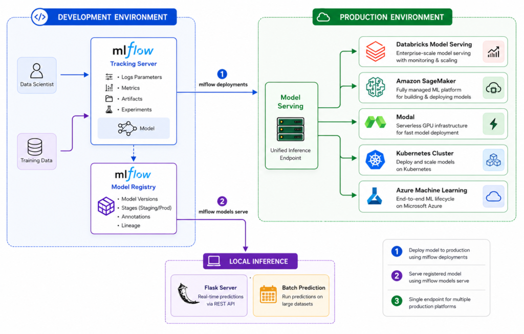
The appropriate deployment architecture depends on how predictions need to be consumed.
| Deployment Pattern | How It Works | Typical Use Cases |
|---|---|---|
| Real-Time REST API | The application sends a request to the model endpoint and immediately receives a prediction. | Fraud detection, recommendation systems, churn scoring |
| Batch Prediction | The model generates predictions for large datasets on a scheduled or on-demand basis. | Customer segmentation, demand forecasting |
| Streaming Prediction | The model continuously processes incoming events or data streams and generates predictions in near real time. | IoT monitoring, anomaly detection, transaction monitoring |
| Edge Deployment | The model runs directly on an edge device instead of relying on a centralized cloud server. | Mobile applications, autonomous vehicles, cameras, industrial devices |
Once we have the model ready, deploying to a local server is straightforward. Use the mlflow models serve command for a one-step deployment. This command starts a local server that listens on the specified port and serves your model.
mlflow models serve -m runs:/<run_id>/model -p 5000We can then send a test request to the server as follows:
curl http://127.0.0.1:5000/invocations -H "Content-Type:application/json" --data '{"inputs": [[1, 2], [3, 4], [5, 6]]}'OR
# Prerequisite: serve a custom pyfunc OpenAI model (not mlflow.openai) on localhost:5678
#   that defines inputs in the below format and params of `temperature` and `max_tokens`

import json
import requests

payload = json.dumps({
    "inputs": {"messages": [{"role": "user", "content": "Tell a joke!"}]},
    "params": {
        "temperature": 0.5,
        "max_tokens": 20,
    },
})
response = requests.post(
    url=f"http://localhost:5678/invocations",
    data=payload,
    headers={"Content-Type": "application/json"},
)
print(response.json())
MLflow uses FastAPI, a modern ASGI web application framework for Python, to serve the inference endpoint. FastAPI handles requests asynchronously and is recognized as one of the fastest Python frameworks. This production-ready framework works well for most use cases.
Instead of running an online inference endpoint, you can execute a single batch inference job on local files using the mlflow models predict command. The following command runs the model prediction on input.csv and outputs the results to output.csv.
# bash
mlflow models predict -m models:/<model_id> -i input.csv -o output.csv
OR
import mlflow

model = mlflow.pyfunc.load_model("models:/<model_id>")
predictions = model.predict(pd.read_csv("input.csv"))
predictions.to_csv("output.csv")Amazon SageMaker provides a fully managed infrastructure for deploying and scaling machine learning inference workloads. MLflow integrates with SageMaker to streamline the deployment of MLflow Models, abstracting much of the container packaging and infrastructure configuration normally required to expose a model as a production inference endpoint.
Amazon SageMaker supports the Bring Your Own Container (BYOC) deployment pattern, allowing custom Docker images to run as managed inference containers. However, a SageMaker-compatible inference container must conform to specific runtime requirements, including a defined container entry point, an HTTP inference server, supported health and invocation endpoints, environment configuration, and model-loading logic.
Implementing these components manually typically requires creating and maintaining a custom Dockerfile, inference server, dependency configuration, and container startup logic.
MLflow simplifies this process by packaging an MLflow Model into a deployment-ready container and orchestrating the required AWS resources. At a high level, the deployment workflow is:
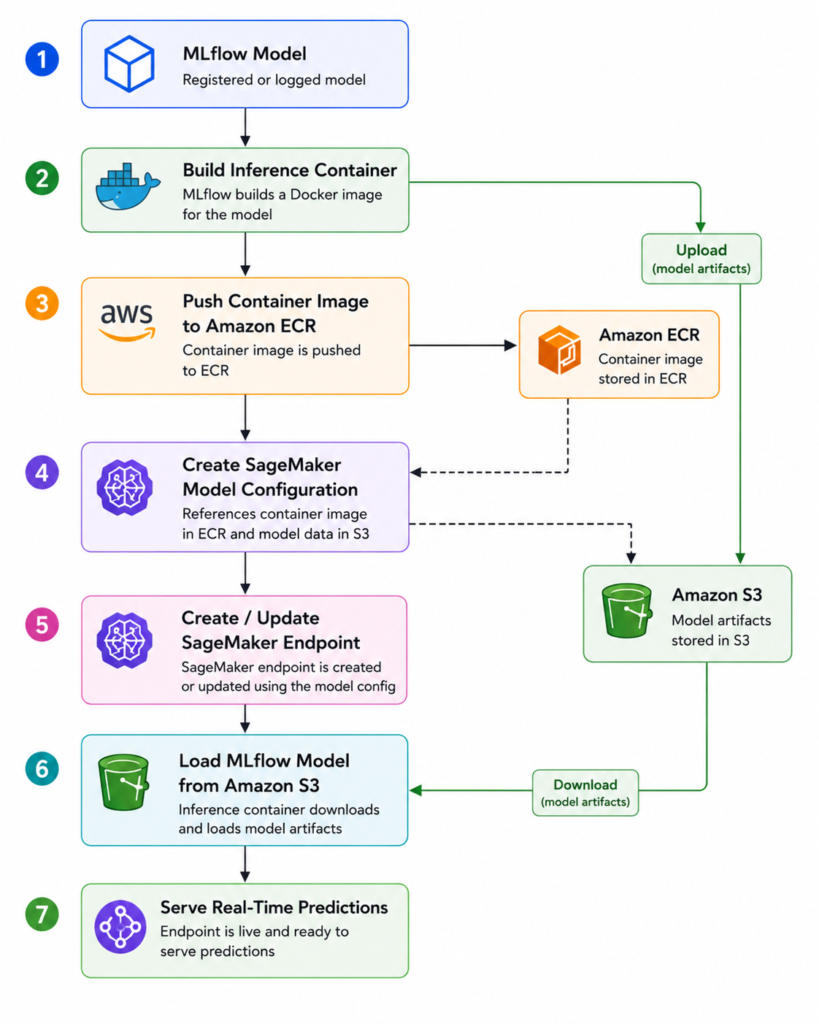
When the SageMaker endpoint starts, the inference container loads the model artifacts and exposes an HTTP-based prediction interface. This provides a consistent serving contract between local MLflow inference and managed SageMaker deployment.
The container provides the same REST endpoints as a local inference server. For instance, the /invocations endpoint accepts CSV and JSON input data and returns prediction results
This abstraction enables teams to move from a registered MLflow Model to a scalable managed inference endpoint without manually implementing the underlying container-serving stack, while still benefiting from SageMaker capabilities such as managed infrastructure, endpoint scaling, monitoring, and production-grade inference hosting.
This section outlines the process of deploying a model to SageMaker using the MLflow CLI.
Install Tools
Ensure the installation of the following tools if not already done:
Permissions Setup
Set up AWS accounts and permissions correctly. We need an IAM role with permissions to create a SageMaker endpoint, access an S3 bucket, and use the ECR repository. This role should also be assumable by the user performing the deployment.
{
  "Version": "2012-10-17",
  "Statement": [
    {
      "Sid": "SageMakerDeployment",
      "Effect": "Allow",
      "Action": [
        "sagemaker:CreateModel",
        "sagemaker:DeleteModel",
        "sagemaker:DescribeModel",
        "sagemaker:CreateEndpointConfig",
        "sagemaker:DeleteEndpointConfig",
        "sagemaker:DescribeEndpointConfig",
        "sagemaker:CreateEndpoint",
        "sagemaker:UpdateEndpoint",
        "sagemaker:DeleteEndpoint",
        "sagemaker:DescribeEndpoint"
      ],
      "Resource": "*"
    },
    {
      "Sid": "ECRAuthentication",
      "Effect": "Allow",
      "Action": [
        "ecr:GetAuthorizationToken"
      ],
      "Resource": "*"
    },
    {
      "Sid": "ECRRepositoryAccess",
      "Effect": "Allow",
      "Action": [
        "ecr:CreateRepository",
        "ecr:DescribeRepositories",
        "ecr:BatchCheckLayerAvailability",
        "ecr:GetDownloadUrlForLayer",
        "ecr:BatchGetImage",
        "ecr:InitiateLayerUpload",
        "ecr:UploadLayerPart",
        "ecr:CompleteLayerUpload",
        "ecr:PutImage"
      ],
      "Resource": "arn:aws:ecr:REGION:ACCOUNT_ID:repository/mlflow-*"
    },
    {
      "Sid": "UploadModelArtifacts",
      "Effect": "Allow",
      "Action": [
        "s3:GetBucketLocation",
        "s3:ListBucket"
      ],
      "Resource": "arn:aws:s3:::YOUR_BUCKET"
    },
    {
      "Sid": "ManageModelArtifacts",
      "Effect": "Allow",
      "Action": [
        "s3:GetObject",
        "s3:PutObject",
        "s3:DeleteObject"
      ],
      "Resource": "arn:aws:s3:::YOUR_BUCKET/*"
    },
    {
      "Sid": "PassSageMakerExecutionRole",
      "Effect": "Allow",
      "Action": [
        "iam:PassRole"
      ],
      "Resource": "arn:aws:iam::ACCOUNT_ID:role/MLflowSageMakerExecutionRole",
      "Condition": {
        "StringEquals": {
          "iam:PassedToService": "sagemaker.amazonaws.com"
        }
      }
    }
  ]
}
Replace REGION, ACCOUNT_ID, and YOUR_BUCKET with your environment-specific values.
The iam:PassRole permission is particularly important: the deployment process creates the SageMaker model and tells SageMaker which execution role it should use.
This is the role that the deployed SageMaker model uses at runtime.
The role should trust the SageMaker service:
{
  "Version": "2012-10-17",
  "Statement": [
    {
      "Effect": "Allow",
      "Principal": {
        "Service": "sagemaker.amazonaws.com"
      },
      "Action": "sts:AssumeRole"
    }
  ]
}It’s recommended to test your model locally before deploying it to a production environment. command deploys the model in a Docker container with an identical image and environment configuration, making it ideal for pre-deployment testing.
$ mlflow deployments run-local -t sagemaker -m models:/<model_id> -p 5000then test the model by sending a POST request to the endpoint:
$ curl -X POST -H "Content-Type:application/json; format=pandas-split" --data '{"columns":["a","b"],"data":[[1,2]]}' http://localhost:5000/invocationsThis command builds a Docker image compatible with SageMaker and uploads it to ECR.
$ mlflow sagemaker build-and-push-container -m models:/<model_id>This command deploys the model to an Amazon SageMaker endpoint. MLflow uploads the Python Function model to S3 and automatically initiates an Amazon SageMaker endpoint serving the model.
$ mlflow deployments create -t sagemaker -m runs:/<run_id>/model \
    -C region_name=<your-region> \
    -C instance-type=ml.m4.xlarge \
    -C instance-count=1 \
-C env='{"DISABLE_NGINX": "true"}''To ensure the model solves a measurable business problem.
To detect issues like schema mismatches, missing values, and invalid data before training.
Data preparation cleans and transforms raw data; feature engineering creates informative inputs for the model.
To estimate how well the model generalizes to unseen data and avoid overfitting.
Model artifacts, metrics, hyperparameters, code version, and dataset version.
Because data and user behavior change over time, causing model performance to degrade.